Adapted from Introduction to Statistical Investigations, AP Version, by Tintle, Chance, Cobb, Rossman, Roy, Swanson and VanderStoep
Bob Lochel, Hatboro-Horsham High School
Before the Thanksgiving break, I started the sampling chapter in AP Statistics. This is a unit filled with new vocabulary and many, many class activities. To get students thinking about random sampling, I have used the "famous" Random Rectangles activity (Google it...you'll find it) and it's cousin - Jelly Blubbers. These activities are effective in causing students to think about the importance of choosing a random sample from a population, and considering communication of procedures. But a new activity I first heard about at a summer session on simulation-based inference, and later explained by Ruth Carver at a recent PASTA meeting, has added some welcome wrinkles to this unit. The unit uses the one-variable sampling applet from the Rossman-Chance applet collection, and is ideal for 1-1 classrooms, or even students working in tech teams. Also, Beth Chance is wonderful...and you should all know that!
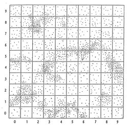
In my classroom notes, students first encounter the "sky", which has been broken into 100 squares. To start, teams work to define procedures for selecting a random sample of 10 squares, using both the "hat" (non-technology) method, and a method using technology (usually a graphing calculator). Before we draw the samples however, I want students to think about the population - specifically, will a random sample do a "good job" with providing estimates? Groups were asked to discuss what they notice about the sky. My classes immediately sensed something worth noting:
"There are some squares where there are many stars (we end up calling these "dense" squares) and some where there are not so many."
Before we even drew our first sample, we are talking about the need to consider both dense and non-dense areas in our sample, and the possibility that our sample will overestimate or underestimate the population, even in random sampling. There's a lot of stats goodness in all of this, and the conversation felt natural and accessible to the students.
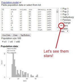
| Students then used their technology-based procedure to actually draw a random sample of 10 squares, marking off the squares. But counting the actual stars is not reasonable, given their quantity - so it's Beth Chance to the rescue! Make sure you click the "stars" population to get started. Beth has provided the number of stars in each square, and information regarding density, row and column to think about later. But before we start clicking blindly, let's describe that population. The class quickly agrees that we have a skewed-right distribution, and take note of the population mean - we'll need it to discuss bias later. |
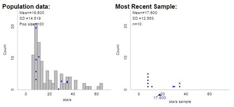
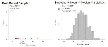
Click "show sampling options" on the top of the screen and we can now simulate random samples. First, students each drew a sample of size 10 - the bottom of the screen shows the sample, summary statistics, and a visual of the 10 squares chosen from the population.
Groups were asked to look at their sample means, share them with neighbors, and think about how close these samples generally come to hitting their target. Find a neighbor where few "dense" area were selected , or where many "dense" squares made the cut, how much confidence do we have in using this procedure to estimate the population mean?
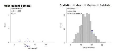
Eventually I unleashed the sampling power of the applet and let students draw more and more samples. And while a formal discussion of sampling distributions is a few chapters away, we can make observations about the distributions of these sample means.
Eventually I unleashed the sampling power of the applet and let students draw more and more samples. And while a formal discussion of sampling distributions is a few chapters away, we can make observations about the distributions of these sample means.
And I knew the discussion was heading in the right direction when a student observed:
"Hey, the population is definitely skewed, but the means are approximately normal. That's odd..."
Yep, it sure is...and more seeds have been planted for later sampling distribution discussions. But what about those dense and non-dense areas the students noticed earlier? Sure, our random samples seem to provide an unbiased estimator of the population mean, but can we do better? This is where Beth's applet is so wonderful, and where this activity separates itself from Random Rectangles. On the top of the applet, we can stratify our sample by density, ensuring that an appropriate ratio of dense / non-dense areas (here, 20%) is maintained in the sample. The applet then uses color to make this distinction clear: here, green dots represent dense-area squares.
Finally, note the reduced variability in the distribution from stratified samples, as opposed to random samples. The payoff is here!
Later, we will look at samples stratified by row and/or column. And cluster samples by row or column will also make an appearance. There's so much to talk about with this one activity, and I appreciate Ruth and Beth for sharing!
Later, we will look at samples stratified by row and/or column. And cluster samples by row or column will also make an appearance. There's so much to talk about with this one activity, and I appreciate Ruth and Beth for sharing!

 RSS Feed